The first part of this course is concerned with:
The choice of design paradigm is an important aspect of algorithm synthesis.
A basic operation could be:
n := 5;
loop
    get(m);
    n := n -1;
until (m=0 or n=0)
Worst-case: 5 iterations
Usually we are not concerned with the number of steps for a single fixed case but wish to estimate the running time in terms of the `input size'.
get(n);
loop
    get(m);
    n := n -1;
until (m=0 or n=0)
Worst-case: n iterations
Sorting:
n == The number of items to be sorted;
Basic operation: Comparison.
Multiplication (of x and y):
n == The number of digits in x plus the number of digits in y.
Basic operations: single digit arithmetic.
Graph `searching':
n == the number of nodes in the graph or the number of edges in the graph.
Time( P ; Q ) = Time( P ) + Time( Q )
Iteration:
while < condition > loop
     P;
end loop;
or
for i in 1..n loop
    P;
end loop
Time = Time( P ) * ( Worst-case number of iterations )
Conditional
if < condition > then
    P;
else
    Q;
end if;
Time  =  Time(P)   if  < condition > =true
         Time( Q ) if  < condition > =false
We shall consider recursive procedures later in the course.
for i in 1..n loop
    for j in 1..n loop
       if i < j then
          swop (a(i,j), a(j,i)); -- Basic operation
       end if;
    end loop;
end loop;
Time  <  n*n*1
       =  n^2
Suppose P, Q and R are 3 algorithms with the following worst-case run times:
| n | P | Q | R |
|---|---|---|---|
| 1 | 1 | 5 | 100 |
| 10 | 1024 | 500 | 1000 |
| 100 | 2 100 | 50,000 | 10,000 |
| 1000 | 2 1000 | 5 million | 100,000 |
If each is run on a machine that executes one million (10^6) operations per second
| n | P | Q | R |
|---|---|---|---|
| 1 | 1(*ms | 5(*ms | 100(*ms |
| 5 | 1 millisec | 0.5 millisec | 1 millisec |
| 100 | 270years | 0.05 secs | 0.01 secs |
| 1000 | 2970years | 5 secs | 0.1 secs |
Thus,
The growth of run-time in terms of n (2^n; n^2; n) is more significant than the exact constant factors (1; 5; 100)
Let f:N-> R and g:N-> R. Then: f( n ) = O( g(n) ) means that
There are values, n0 and c, such that f( n ) < = c * g( n ) whenever n > = n0.
Thus we can say that an algorithm has, for example,
Again let, f:N-> R and g:N-> R. Then: f( n ) = OM ( g(n) ) means that there are values, n0 and c, such that f( n ) > = c * g( n ) whenever n > = n0.
Again let, f:N-> R and g:N-> R.
If f(n)=O(g(n)) and f(n)=OM(g(n))
Then we write, f( n ) = THETA ( g(n) )
In this case, f(n) is said to be asymptotically equal to g(n).
If f( n ) = THETA( g(n) ) then algorithms with running times f(n) and g(n) appear to perform similarly as n gets larger.
f(n)=O(g(n)) if and only if g(n)=OM(f(n))
If f(n) = O(g(n)) then
f(n)+g(n)=O(g(n)) ; f(n)+g(n)=OM(g(n))
f(n)*g(n)=O(g(n)^2) ; f(n)*g(n)=OM(f(n)^2)
Suppose f(n)=10n and g( n )=2n^2
This is a method of designing algorithms that (informally) proceeds as follows:
Given an instance of the problem to be solved, split this into several, smaller, sub-instances (of the same problem) independently solve each of the sub-instances and then combine the sub-instance solutions so as to yield a solution for the original instance. This description raises the question:
By what methods are the sub-instances to be independently solved?
The answer to this question is central to the concept of Divide-&-Conquer algorithm and is a key factor in gauging their efficiency.
Consider the following: We have an algorithm, alpha say, which is known to solve all problem instances of size n in at most c n^2 steps (where c is some constant). We then discover an algorithm, beta say, which solves the same problem by:
T(alpha)( n ) = Running time of alpha
T(beta)( n ) = Running time of beta
Then,
T(alpha)( n ) = c n^2 (by definition of alpha)
But
T(beta)( n )  = 3 T(alpha)( n/2 ) + d n

              = (3/4)(cn^2) + dn
So if dn < (cn^2)/4 (i.e. d < cn/4) then beta is faster than alpha
In particular for all large enough n, (n > 4d/c = Constant), beta is faster than alpha.
This realisation of beta improves upon alpha by just a constant factor. But if the problem size, n, is large enough then
         n     >   4d/c
         n/2   >   4d/c
               ...
         n/2^i >   4d/c
which suggests that using beta instead of alpha for the `solves these' stage repeatedly until the sub-sub-sub..sub-instances are of size n0 < = (4d/c) will yield a still faster algorithm.
So consider the following new algorithm for instances of size n
procedure gamma (n : problem size ) is
   begin
       if n <= n^-0 then
           Solve problem using Algorithm alpha;
        else
           Split into 3 sub-instances of size n/2;
           Use gamma to solve each sub-instance;
           Combine the 3 sub-solutions;
        end if;
   end gamma;
Let T(gamma)(n) denote the running time of this algorithm.
                cn^2                  if n < = n0
T(gamma)(n)  =
                3T(gamma)( n/2 )+dn   otherwise
We shall show how relations of this form can be estimated later in the course. With these methods it can be shown that
T(gamma)( n ) = O( n^{log3} ) (=O(n^{1.59..})
This is an asymptotic improvement upon algorithms alpha and beta.
The improvement that results from applying algorithm gamma is due to the fact that it maximises the savings achieved beta.
The (relatively) inefficient method alpha is applied only to "small" problem sizes.
The precise form of a divide-and-conquer algorithm is characterised by:
In (II) it is more usual to consider the ratio of initial problem size to sub-instance size. In our example this was 2. The threshold in (I) is sometimes called the (recursive) base value. In summary, the generic form of a divide-and-conquer algorithm is:
procedure D-and-C (n : input size) is
   begin
      if n < = n0 then
         Solve problem without further
         sub-division;
       else
          Split into r sub-instances
          each of size n/k;
          for each of the r sub-instances do
            D-and-C (n/k);
          Combine the r resulting
          sub-solutions to produce
          the solution to the original problem;
       end if;
    end D-and-C;
Such algorithms are naturally and easily realised as:
Consider the following problem: one has a directory containing a set of names and a telephone number associated with each name.
The directory is sorted by alphabetical order of names. It contains n entries which are stored in 2 arrays:
names (1..n) ; numbers (1..n)
Given a name and the value n the problem is to find the number associated with the name.
We assume that any given input name actually does occur in the directory, in order to make the exposition easier.
The Divide-&-Conquer algorithm to solve this problem is the simplest example of the paradigm.
It is based on the following observation
Given a name, X say,
X occurs in the middle place of the names array
Or
X occurs in the first half of the names array. (U)
Or
X occurs in the second half of the names array. (L)
U (respectively L) are true only if X comes before (respectively after) that name stored in the middle place.
This observation leads to the following algorithm:
function search (X : name;
                             start, finish : integer)
                             return integer is
   middle : integer;
   begin
      middle := (start+finish)/2;
      if names(middle)=x then
          return numbers(middle);
      elsif X<names(middle) then
          return search(X,start,middle-1);
      else -- X>names(middle)
          return search(X,middle+1,finish);
      end if;
   end search;
Exercise: How should this algorithm be modified to cater for the possibility that a given name does not occur in the directory? In terms of the generic form of divide-&-conquer algorithms, at which stage is this modification made?
We defer analysis of the algorithm's performance until later.
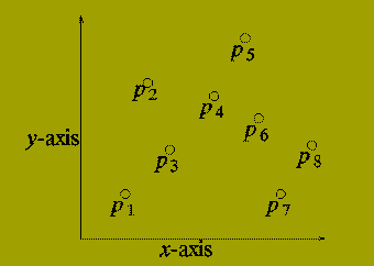
P = {p(1), p(2) ,..., p(n) }
where p(i) = ( x(i), y(i) ).
A set of n points in the plane.
Output
The distance between the two points that are closest.
Note: The distance DELTA( i, j ) between p(i) and p(j) is defined by the expression:
Square root of { (x(i)-x(j))^2 + (y(i)-y(j))^2 }
We describe a divide-and-conquer algorithm for this problem.
We assume that:
n is an exact power of 2, n = 2^k.
For each i, x(i) < = x(i+1), i.e. the points are ordered by increasing x from left to right.
Consider drawing a vertical line (L) through the set of points P so that half of the points in P lie to the left of L and half lie to the right of L.
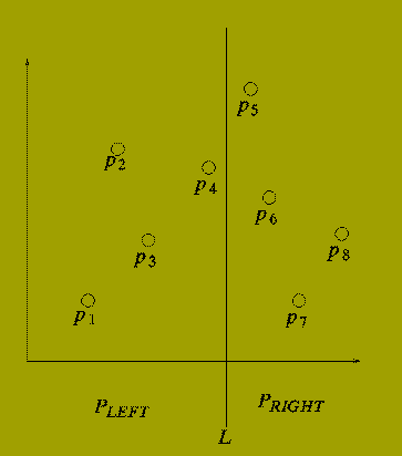
There are three possibilities:
One Point from P-LEFT
and
One Point from P-RIGHT
So we have a (rough) Divide-and-Conquer Method as follows:
function closest_pair (P: point set; n: in
teger )
                               return float is
   DELTA-LEFT, DELTA-RIGHT : float;
   DELTA : float;
   begin
      if n = 2 then
         return distance from p(1) to p(2);
      else
         P-LEFT  := ( p(1), p(2) ,..., p(n/2) );
         P-RIGHT := ( p(n/2+1), p(n/2+2) ,..., p(n) );
         DELTA-LEFT := closestpair( P-LEFT, n/2 );
         DELTA-RIGHT := closestpair( P-RIGHT, n/2 );
         DELTA := minimum ( DELTA-LEFT, DELTA-RIGHT );
         --*********************************************
         Determine whether there are points p(l) in
         P-LEFT and p(r) in P-RIGHT with
         distance( p(l), p(r) ) < DELTA. If there
         are such points, set DELTA to be the smallest
         distance.
         --**********************************************
         return DELTA;
      end if;
end closest_pair;
The section between the two comment lines is the `combine' stage of the Divide-and-Conquer algorithm.
If there are points p(l) and p(r) whose distance apart is less than DELTA then it must be the case that
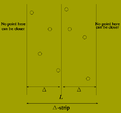
The combine stage can be implemented by:
Call the set of points found in (1) and (2) P-strip. and sort the s points in this in order of increasing y-coordinate. letting ( q(1),q(2) ,..., q(s) ) denote the sorted set of points.
Then the combine stage of the algorithm consists of two nested for loops:
for i in 1..s loop
   for j in i+1..s loop
      exit when (| x(i) - x(j) | > DELTA or
                       | y(i) - y(j) | > DELTA);
       if distance( q(i), q(j) ) < DELTA then
          DELTA := distance ( q(i), q(j) );
       end if;
   end loop;
end loop;
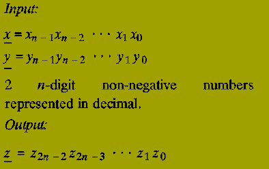
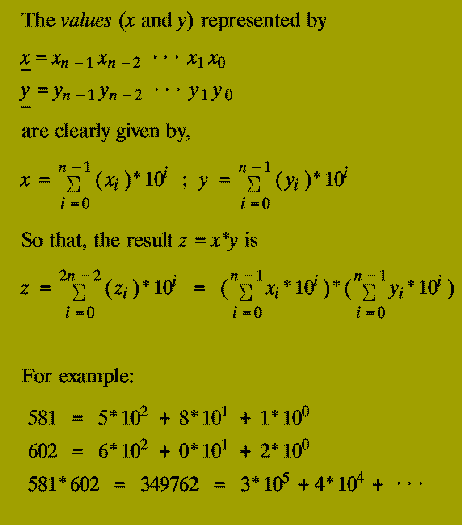
The (2n)-digit decimal representation of the product x * y.
Note: The algorithm below works for any number base, e.g. binary, decimal, hexadecimal, etc. We use decimal simply for convenience.
The classical primary school algorithm for multiplication requires O( n^2 ) steps to multiply two n-digit numbers.
A step is regarded as a single operation involving two single digit numbers, e.g. 5+6, 3*4, etc.
In 1962, A.A. Karatsuba discovered an asymptotically faster algorithm for multiplying two numbers by using a divide-and-conquer approach.
From this we also know that the result of multiplying x and y (i.e. z) is
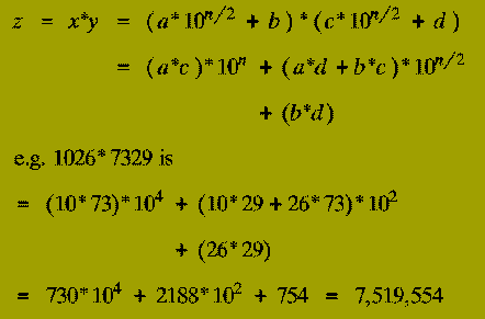
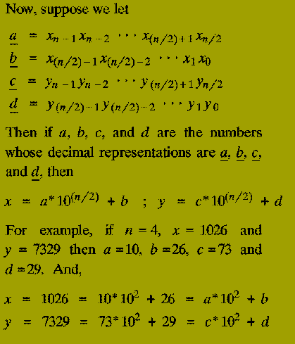
The terms ( a*c ), ( a*d ), ( b*c ), and ( b*d ) are each products of
Thus the expression for the multiplication of x and y in terms of the numbers a, b, c, and d tells us that:
(1-3) therefore describe a Divide-&-Conquer algorithm for multiplying two n-digit numbers represented in decimal. However,
Moderately difficult: How many steps does the resulting algorithm take to multiply two n-digit numbers?
Karatsuba discovered how the product of 2 n-digit numbers could be expressed in terms of three products each of 2 (n/2)-digit numbers - instead of the four products that a naive implementation of the Divide-and-Conquer schema above uses.
This saving is accomplished at the expense of slightly increasing the number of steps taken in the `combine stage' (Step 3) (although, this will still only use O( n ) operations).
Suppose we compute the following 3 products (of 2 (n/2)-digit numbers):
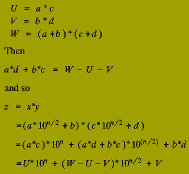
function Karatsuba (xunder, yunder : n-digit integer;
                           n : integer)
                           return (2n)-digit integer is
a, b, c, d : (n/2)-digit integer
U, V, W : n-digit integer;
begin
   if n = 1 then
      return x(0)*y(0);
   else
      a := x(n-1) ... x(n/2);
      b := x(n/2-1) ... x(0);
      c := y(n-1) ... y(n/2);
      d := y(n/2-1) ... y(0);
      U := Karatsuba ( a, c, n/2 );
      V := Karatsuba ( b, d, n/2 );
      W := Karatsuba ( a+b, c+d, n/2 );
      return U*10^n + (W-U-V)*10^n/2 + V;
   end if;
 end Karatsuba;
This is useful in allowing comparisons between the performances of two algorithms to be made.
For Divide-and-Conquer algorithms the running time is mainly affected by 3 criteria:
Suppose, P, is a divide-and-conquer algorithm that instantiates alpha sub-instances, each of size n/beta.
Let Tp( n ) denote the number of steps taken by P on instances of size n. Then
Tp( n0 )  =  Constant   (Recursive-base)
Tp( n )   =  alpha Tp( n/beta ) + gamma( n )
In the case when alpha and beta are both constant (as in all the examples we have given) there is a general method that can be used to solve such recurrence relations in order to obtain an asymptotic bound for the running time Tp( n ).
In general:
T( n ) = alpha T( n/beta ) + O( n^gamma )
(where gamma is constant) has the solution
            O(n^gamma)             if   alpha < beta^gamma
T( n )  =   O(n^gamma log n)       if   alpha = beta^gamma}
            O(n^{log^-beta(alpha)) if   alpha > beta^gamma
This paradigm is most often applied in the construction of algorithms to solve a certain class of
That is: problems which require the minimisation or maximisation of some measure.
One disadvantage of using Divide-and-Conquer is that the process of recursively solving separate sub-instances can result in the same computations being performed repeatedly since identical sub-instances may arise.
The idea behind dynamic programming is to avoid this pathology by obviating the requirement to calculate the same quantity twice.
The method usually accomplishes this by maintaining a table of sub-instance results.
Dynamic Programming is a
in which the smallest sub-instances are explicitly solved first and the results of these used to construct solutions to progressively larger sub-instances.
In contrast, Divide-and-Conquer is a
which logically progresses from the initial instance down to the smallest sub-instances via intermediate sub-instances. We can illustrate these points by considering the problem of calculating the Binomial Coefficient, "n choose k", i.e.
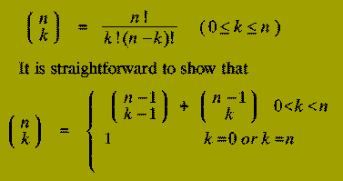
Using this relationship, a rather crude Divide-and-Conquer solution to the problem of calculating the Binomial Coefficient `n choose k' would be:
function bin_coeff (n : integer;
                                k : integer)
                                return integer is
   begin
      if k = 0 or k = n then
         return 1;
      else
         return
         bincoeff(n-1, k-1) + bincoeff(n-1, k);
      end if;
   end bin_coeff;
By contrast, the Dynamic Programming approach uses the same relationship but constructs a table of all the (n+1)*(k+1) binomial coefficients `i choose j' for each value of i between 0 and n, each value of j between 0 and k.
These are calculated in a particular order:
(i-1)+(j-1) < (i-1)+j < i+j
The Dynamic Programming method is given by:
function bin_coeff (n : integer;
                                k : integer)
                                return integer is
type table is array (0..n, 0..k) of integer;
bc : table;
i, j, k : integer;
sum : integer;
begin
   for i in 0..n loop
     bc(i,0) := 1;
   end loop;
   bc(1,1) := 1;
   sum := 3; i := 2; j := 1;
   while sum <= n+k loop
      bc(i,j) := bc(i-1,j-1)+bc(i,j-1);
      i := i-1; j := j+1;
      if i < j or j > k then
         sum := sum + 1;
         if sum <= n+1 then
            i := sum-1; j := 1;
         else
            i := n; j := sum-n;
         end if;
      end if;
    end loop;
   return bc(n,k);
end bin_coeff;
The section of the function consisting of the lines:
if i < j or j > k then
   sum := sum + 1;
   if sum <= n+1 then
      i := sum-1; j := 1;
   else
      i := n; j := sum-n;
   end if;
end if;
is invoked when all the table entries `i choose j', for which i+j equals the current value of sum, have been found. The if statement increments the value of sum and sets up the new values of i and j.
Now consider the differences between the two methods: The Divide-and-Conquer approach recomputes values, such as "2 choose 1", a very large number of times, particularly if n is large and k depends on n, i.e. k is not a constant.
It can be shown that the running time of this method is
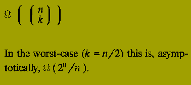
Despite the fact that the algorithm description is quite simple (it is just a direct implementation of the relationship given) it is completely infeasible as a practical algorithm.
The Dynamic Programming method, since it computes each value "i choose j" exactly once is far more efficient. Its running time is O( n*k ), which is O( n^2 ) in the worst-case, (again k = n/2).
It will be noticed that the dynamic programming solution is rather more involved than the recursive Divide-and-Conquer method, nevertheless its running time is practical.
The binomial coefficient example illustrates the key features of dynamic programming algorithms.
Input: A directed graph, G( V, E ), with nodes
V = {1, 2 ,..., n }
and edges E as subset of VxV. Each edge in E has associated with it a non-negative length.
Output: An nXn matrix, D, in which D^(i,j) contains the length of the shortest path from node i to node j in G.
The algorithm, conceptually, constructs a sequence of matrices:
D0, D1 ,..., Dk ,..., Dn
For each k (with 1 < = k < = n), the (i, j) entry of Dk, denoted Dk( i,j ), will contain the Length of the shortest path from node i to node j when only the nodes
can be used as intermediate nodes on the path.
Obviously Dn = D.
The matrix, D0, corresponds to the `smallest sub-instance'. D0 is initiated as:
               0  if i=j
D0( i, j )  =  infinite  if (i,j) not in E
               Length(i,j)  if (i,j) is in E
Now, suppose we have constructed Dk, for some k < n.
How do we proceed to build D(k+1)?
The shortest path from i to j with only
Either: Does not contain the node k+1.
Or: Does contain the node k+1.
In the former case:
D(k+1)( i, j ) = Dk( i, j )
In the latter case:
D(k+1)( i, j ) = D-k( i, k+1 ) + D-k( k+1, j )
Therefore D(k+1)( i, j ) is given by
                       Dk(i,j)
               minimum
                       Dk( i, k+1 ) + Dk( k+1, j )
Although these relationships suggest using a recursive algorithm, as with the previous example, such a realisation would be extremely inefficient.
Instead an iterative algorithm is employed.
Only one nXn matrix, D, is needed.
This is because after the matrix D(k+1) has been constructed, the matrix Dk is no longer needed. Therefore D(k+1) can overwrite Dk.
In the implementation below, L denotes the matrix of edge lengths for the set of edges in the graph G( V, E ).
type matrix is array (1..n, 1..n) of integer;
L : matrix
function shortest_path_length (L : matrix;
                                   n : integer)
                                   return matrix is
D : matrix; -- Shortest paths matrix
begin
  -- Initial sub-instance
  D(1..n,1..n) := L(1..n,1..n);
  for k in 1..n loop
    for i in 1..n loop
      for j in 1..n loop
        if D(i,j) > D(i,k) + D(k,j) then
           D( i,j ) := D(i,k) + D(k,j);
        end if;
      end loop;
    end loop;
  end loop;
  return D(1..n,1..n);
end shortest_path_length;
This algorithm, discovered by Floyd, clearly runs in time
Thus O( n ) steps are used to compute each of the n^2 matrix entries.
All Greedy Algorithms have exactly the same general form. A Greedy Algorithm for a particular problem is specified by describing the predicates `solution' and `feasible'; and the selection function `select'.
Consequently, Greedy Algorithms are often very easy to design for optimisation problems.
The General Form of a Greedy Algorithm is
function select (C : candidate_set) return candidate;
function solution (S : candidate_set) return
boolean;
function feasible (S : candidate_set) return
boolean;
--***************************************************
function greedy (C : candidate_set) return candidate_set is
x : candidate;
S : candidate_set;
begin
   S := {};
   while (not solution(S)) and C /= {} loop
     x := select( C );
     C := C - {x};
     if feasible( S union {x} ) then
        S := S union { x };
     end if;
   end loop;
   if solution( S ) then
     return S;
   else
     return es;
   end if;
end greedy;
As illustrative examples of the greedy paradigm we shall describe algorithms for the following problems:
The inputs for this problem is an (undirected) graph, G( V, E ) in which each edge, e in E, has an associated positive edge length, denoted Length( e ).
The output is a spanning tree, T( V, F ) of G( V,E ) such that the total edge length, is minimal amongst all the possible spanning trees of G( V,E ).
Note: An n-node tree, T is a connected n-node graph with exactly n-1 edges.
T( V,F ) is a spanning tree of G( V,E ) if and only if T is a tree and the edges in F are a subset of the edges in E.
In terms of general template given previously:
function min_spanning_tree (E : edge_set)
                           return edge_set is
S : edge_set;
e : edge;
begin
  S := (es;
  while (H(V,S) not a tree)
               and E /= {} loop
    e :=  Shortest edge in E;
    E := E - {e};
    if H(V, S union {e}) is acyclic then
      S := S union {e};
    end if;
   end loop;
   return S;
end min_spanning_tree;
Before proving the correctness of this algorithm, we give an
example of it running.
The algorithm may be viewed as dividing the set of nodes, V, into n parts or components:
{1} ; {2} ; ... ; {n}
An edge is added to the set S if and only if it joins two nodes which belong to different components; if an edge is added to S then the two components containing its endpoints are coalesced into a single component.
In this way, the algorithm stops when there is just a single component
{ 1, 2 ,..., n }
remaining.
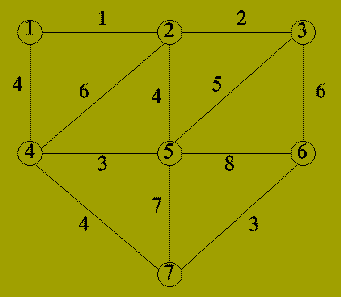
| Iteration | Edge | Components |
|---|---|---|
| 0 | - | {1}; {2}; {3}; {4}; {5}; {6}; {7} |
| 1 | {1,2} | {1,2}; {3}; {4}; {5}; {6}; {7} |
| 2 | {2,3} | {1,2,3}; {4}; {5}; {6}; {7} |
| 3 | {4,5} | {1,2,3}; {4,5}; {6}; {7} |
| 4 | {6,7} | {1,2,3}; {4,5}; {6,7} |
| 5 | {1,4} | {1,2,3,4,5}; {6,7} |
| 6 | {2,5} | Not included (adds cycle) |
| 7 | {4,7} | {1,2,3,4,5,6,7} |
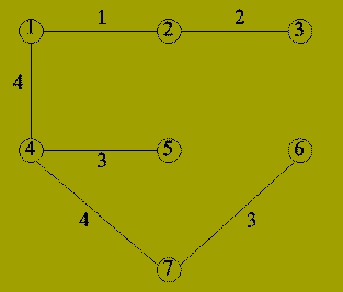
Question: How do we know that the resulting set of edges form a Minimal Spanning Tree?
In order to prove this we need the following result.
For G(V,E) as before, a subset, F, of the edges E is called promising if F is a subset of the edges in a minimal spanning tree of G(V,E).
Lemma: Let G(V,E) be as before and W be a subset of V.
Let F, a subset of E be a promising set of edges such that no edges in F has exactly one endpoint in W.
If {p,q} in E-F is a shortest edge having exactly one of p or q in W then: the set of edges F union { {p,q} } is promising.
Proof: Let T(V,H) be a minimal spanning tree of G(V,E) such that F is a subset of H. Note that T exists since F is a promising set of edges.
Consider the edge e = {p,q} of the Lemma statement.
If e is in H then the result follows immediately, so suppose that e is not in H. Assume that p is in W and q is not in W and consider the graph T(V, H union {e}).
Since T is a tree the graph T (which contains one extra edge) must contain a cycle that includes the (new) edge {p,q}.
Now since p is in W and q is not in W there must be some edge, e' = {p',q'} in H which is also part of this cycle and is such that p' is in W and q' is not in W.
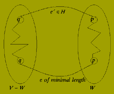
Now, by the choice of e, we know that
Length ( e ) < = Length ( e' )
Removing the edge e' from T gives a new spanning tree of G(V,E).
The cost of this tree is exactly
cost( T ) - Length(e') + Length(e)
and this is < = cost(T).
T is a minimal spanning tree so either e and e' have the same length or this case cannot occur. It follows that there is a minimal spanning tree containing F union {e} and hence this set of edges is promising as claimed.
Theorem: Kruskal's algorithm always produces a minimal spanning tree.
Proof: We show by induction on k > = 0 - the number of edges in S at each stage - that the set of edges in S is always promising.
Base (k = 0): S = {} and obviously the empty set of edges is promising.
Step: (< = k-1 implies k): Suppose S contains k-1 edges. Let e = {p,q} be the next edge that would be added to S. Then:
In various forms this is a frequently arising optimisation problem. Input: A set of items U = {u1, u2 ,..., uN}
each item having a given size s( ui ) and value v( ui ).
A capacity K.
Output: A subset B of U such that the sum over u in B of s(u) does not exceed K and the sum over u in B of v(u) is maximised.
No fast algorithm guaranteed to solve this problem has yet been discovered.
It is considered extremely improbable that such an algorithm exists.
Using a greedy approach, however, we can find a solution whose value is at worst 1/2 of the optimal value.
The selection function chooses that item, ui for which
                    v( ui )
                   --------
                    s( ui )
is maximal
These yield the following greedy algorithm which approximately solves the integer knapsack problem.
function knapsack (U : item_set;
                          K : integer )
                          return item_set is
C, S : item_set;
x : item;
begin
   C := U; S := {};
   while C /= {} loop
      x := Item u in C such that
             v(u)/s(u) is largest;
      C := C - {x};
      if ( sum over {u in S} s(u) ) + s(x) < = K then
         S := S union {x};
      end if;
   end loop;
   return S;
end knapsack;
A very simple example shows that the method can fail to deliver an optimal solution. Let
U = { u1, u2, u3 ,..., u12 }
s(u1) = 101 ; v(u1) = 102
s(ui) = v(ui) = 10 2 < = i < = 12
K = 110
Greedy solution: S = {u1}; Value is 102.
Optimal solution: S = U - {u1}; Value is 110.
In a number of applications graph structures occur. The graph may be an explicit object in the problem instance as in:
Graphs, however, may also occur implicitly as an abstract mechanism with which to analyse problems and construct algorithms for these. Among the many areas where such an approach has been used are:
Whether a graph is an explicit or implicit structure in describing a problem, it is often the case that searching the graph structure may be necessary. Thus it is required to have methods which
That is to say, (With the exception of the first node inspected)
Any new node examined must be adjacent to some node that has previously been visited.
So, search methods implicitly describe an ordering of the nodes in a given graph.
One search method that occurs frequently with implicit graphs is the technique known as
Suppose a problem may be expressed in terms of detecting a particular class of subgraph in a graph.
Then the backtracking approach to solving such a problem would be:
Scan each node of the graph, following a specific order, until
Given a natural number, n, describe how a Knight should be moved on an n times n chessboard so that it visits every square exactly once and ends on its starting square.
The implicit graph in this problem has n^2 nodes corresponding to each position the Knight must occupy. There is an edge between two of these nodes if the corresponding positions are `one move apart'. The sub-graph that defines a solution is a cycle which contains each node of the implicit graph.
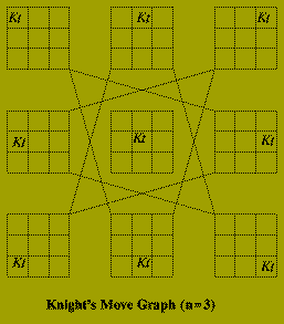
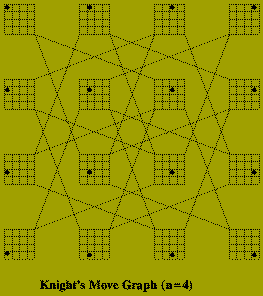
Of course it is not necessary to construct this graph explicitly, in order to to solve the problem. The algorithm below, recursively searches the graph, labeling each square (i.e. node) in the order in which it is visited. In this algorithm:
type chess_board is array (1..n,1..n) of integer;
procedure knight (board : in out chess_board;
                         x,y,move : in out integer;
                         ok : in out boolean) is
w, z : integer;
begin
   if move = n^2+1 then
     ok := ( (x,y) = (1,1) );
   elsif board(x,y) /= 0 then
     ok := false;
   else
     board(x,y) := move;
     loop
       (w,z) := Next position from (x,y);
       knight(board, w, z, move+1, ok );
       exit when (ok or No moves remain);
     end loop;
     if not ok then
       board ( x,y ) :=0; -- Backtracking
     end if;
    end if;
end knight;
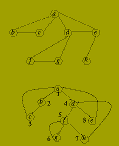
Depth-first search is one method of constructing a search tree for explicit graphs.
Let G(V,E) be a connected graph. A search tree of G(V,E) is a spanning tree, T(V, F) of G(V,E) in which the nodes of T are labelled with unique values k (1 < = k < = |V|) which satisfy:
Given an undirected graph G(V,E), the depth-first search method constructs a search tree using the following recursive algorithm.
procedure depth_first_search (G(V,E) : graph;
                                v : node;
                                lambda : integer;
                                T : in outsearch_tree) is
begin
   label(v) := lambda;
   lambda := lambda+1;
   for each w such that {v,w} mem E loop
     if label(w) = 0 then
       Add edge {v,w} to T;
       depth_first_search(G(V,E),w,lambda,T);
     end if;
   end loop;
end depth_fist_search;
--*******************************
-- Main Program Section
--******************************
begin
   for w mem V loop
     label( w ) := 0;
   end loop;
   lambda := 1;
   depthfirstsearch ( G(V,E), v, lambda, T);
end;
If G( V,E ) is a directed graph then it is possible that not all of the nodes of the graph are reachable from a single root node. To deal with this the algorithm is modified by changing the `Main Program Section' to
begin
  for each w in V loop
    label( w ) := 0;
  end loop;
  lambda := 1;
  for each v mem V loop
    if label( v ) = 0 then
      depthfirstsearch ( G(V,E),v,lambda,T );
    end if;
  end loop;
end;
The running time of both algorithms, input G( V,E ) is O( |E| ) since each edge of the graph is examined only once.
It may be noted that the recursive form given, is a rather inefficient method of implementing depth first search for explicit graphs.
Iterative versions exist, e.g. the method of Hopcroft and Tarjan which is based on a 19th century algorithm discovered by Tremaux. Depth-first search has a large number of applications in solving other graph based problems, for example:
Planarity Testing
One disadvantage of depth first search as a mechanism for searching implicit graph structures, is that expanding some paths may result in the search process never terminating because no solution can be reached from these. For example this is a possible difficulty that arises when scanning proof trees in Prolog implementations.
Breadth-first Search is another search method that is less likely to exhibit such behaviour.
lambda := 1; -- First label
CurrentLevel := {v}; -- Root node
while CurrentLevel /= (es loop
  for each v mem CurrentLevel loop
    NextLevel := Nextlevel union
                 Unmarked neighbours of v;
    if label( v ) = 0 then
      label( v ) := lambda;
      lambda := lambda + 1;
    end if;
  end loop;
  CurrentLevel := NextLevel;
  NextLevel := (es;
end loop;
Thus each vertex labelled on the k'th iteration of the outer loop is `expanded' before any vertex found later.